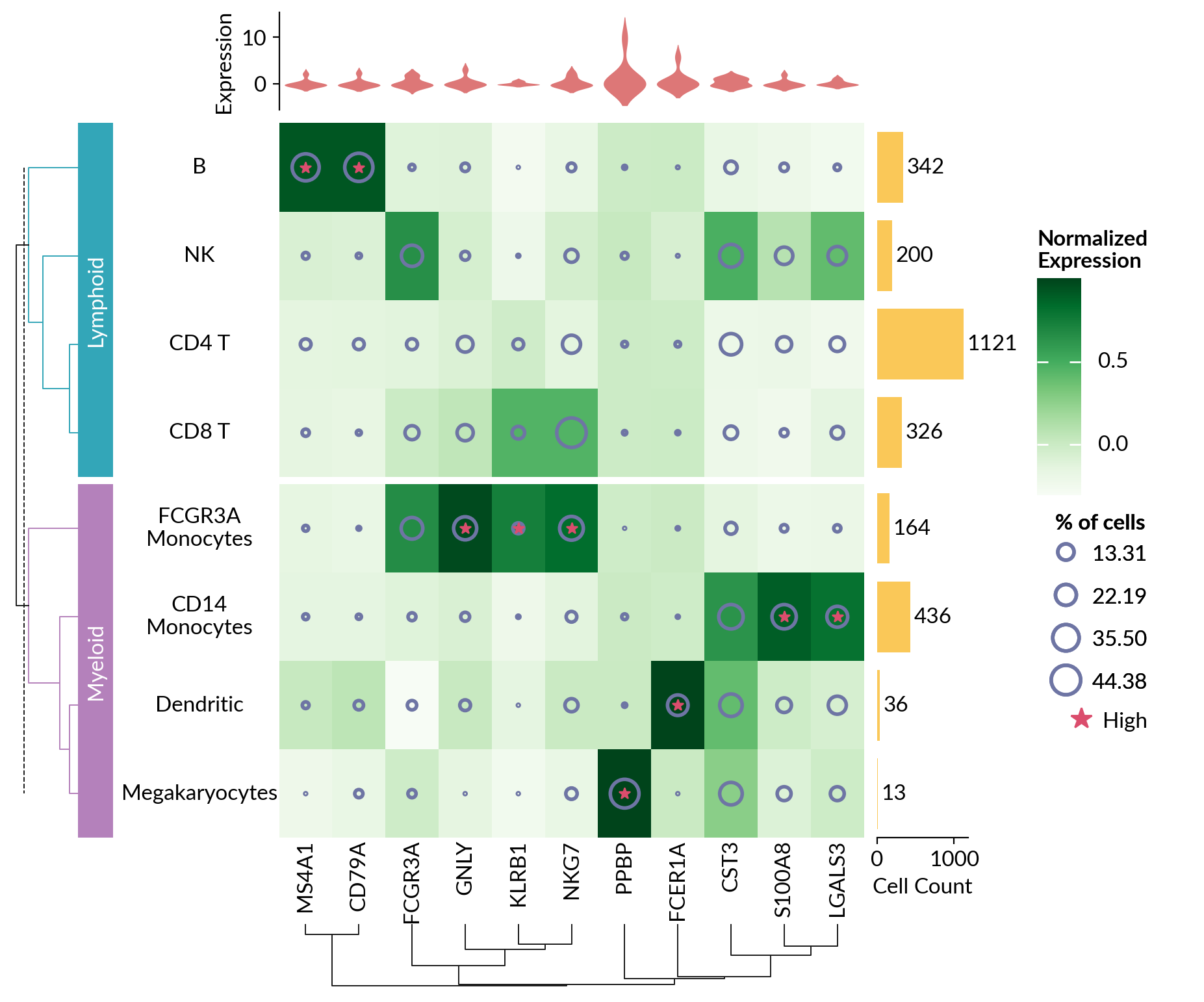
Visualizing Single-cell RNA-seq Data

import matplotlib as mpl
import matplotlib.pyplot as plt
from matplotlib.colors import Normalize
import marsilea as ma
import marsilea.plotter as mp

from sklearn.preprocessing import normalize


pbmc3k = ma.load_data("pbmc3k")
exp = pbmc3k["exp"]
pct_cells = pbmc3k["pct_cells"]
count = pbmc3k["count"]

matrix = normalize(exp.to_numpy(), axis=0)

cell_cat = [
    "Lymphoid",
    "Myeloid",
    "Lymphoid",
    "Lymphoid",
    "Lymphoid",
    "Myeloid",
    "Myeloid",
    "Myeloid",
]
cell_names = [
    "CD4 T",
    "CD14\nMonocytes",
    "B",
    "CD8 T",
    "NK",
    "FCGR3A\nMonocytes",
    "Dendritic",
    "Megakaryocytes",
]

# Make plots
cells_proportion = mp.SizedMesh(
    pct_cells,
    size_norm=Normalize(vmin=0, vmax=100),
    color="none",
    edgecolor="#6E75A4",
    linewidth=2,
    sizes=(1, 600),
    size_legend_kws=dict(title="% of cells", show_at=[0.3, 0.5, 0.8, 1]),
)
mark_high = mp.MarkerMesh(matrix > 0.7, color="#DB4D6D", label="High")
cell_count = mp.Numbers(count["Value"], color="#fac858", label="Cell Count")
cell_exp = mp.Violin(
    exp, label="Expression", linewidth=0, color="#ee6666", density_norm="count"
)
cell_types = mp.Labels(cell_names, align="center")
gene_names = mp.Labels(exp.columns)

# Group plots together
h = ma.Heatmap(
    matrix, cmap="Greens", label="Normalized\nExpression", width=4.5, height=5.5
)
h.add_layer(cells_proportion)
h.add_layer(mark_high)
h.add_right(cell_count, pad=0.1, size=0.7)
h.add_top(cell_exp, pad=0.1, size=0.75, name="exp")
h.add_left(cell_types)
h.add_bottom(gene_names)

h.group_rows(cell_cat, order=["Lymphoid", "Myeloid"])
h.add_left(mp.Chunk(["Lymphoid", "Myeloid"], ["#33A6B8", "#B481BB"]), pad=0.05)
h.add_dendrogram("left", colors=["#33A6B8", "#B481BB"])
h.add_dendrogram("bottom")
h.add_legends("right", align_stacks="center", align_legends="top", pad=0.2)
h.set_margin(0.2)
h.render()

# h.get_ax("exp").set_yscale("symlog")