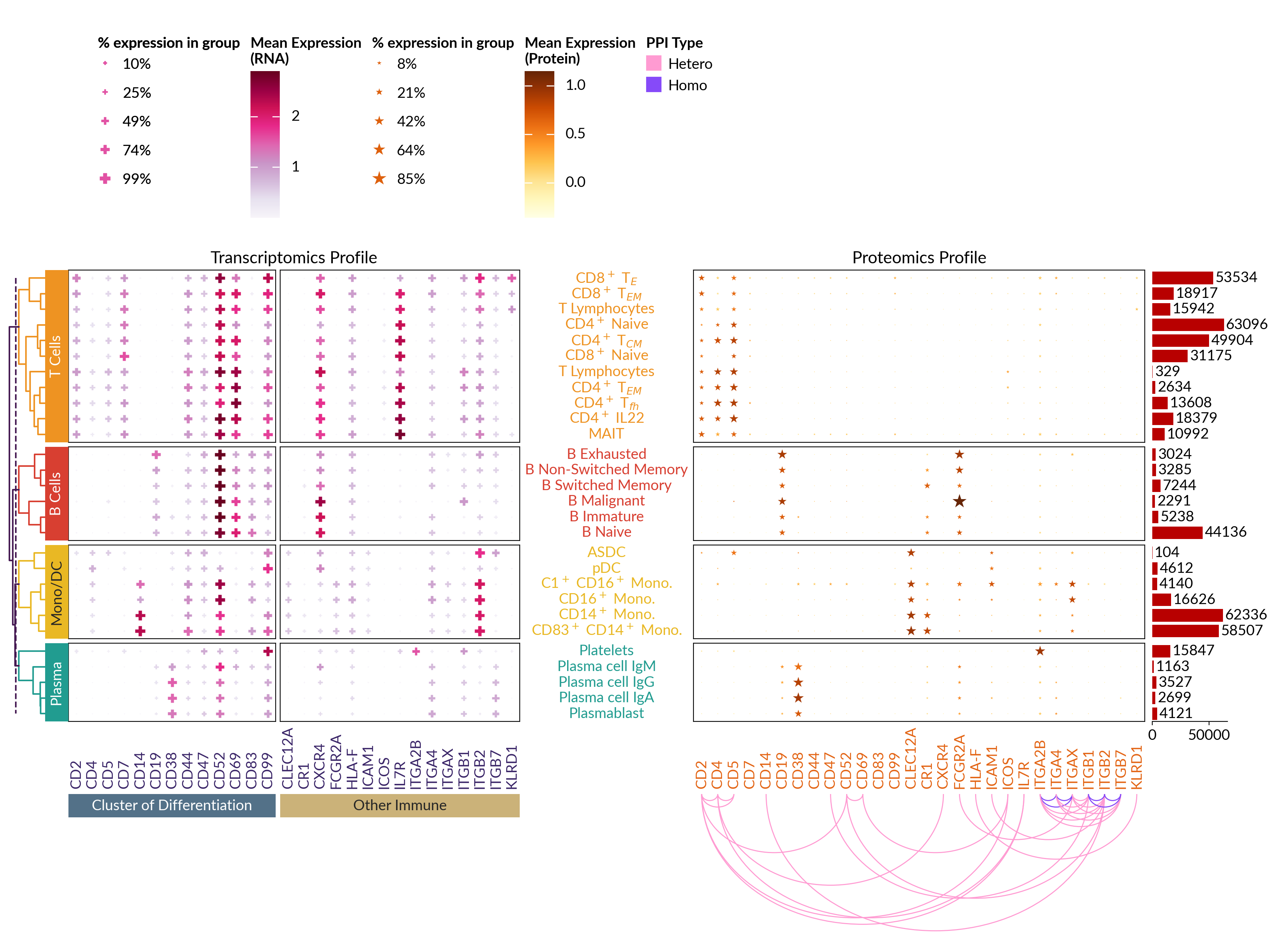
Visualizing Single-cell Multi-Omics Data

import matplotlib as mpl
from matplotlib.ticker import FuncFormatter


import marsilea as ma

dataset = ma.load_data("sc_multiomics")

fmt = FuncFormatter(lambda x, _: f"{x:.0%}")
lineage = ["B Cells", "T Cells", "Mono/DC", "Plasma"]
lineage_colors = ["#D83F31", "#EE9322", "#E9B824", "#219C90"]
m = dict(zip(lineage, lineage_colors))
cluster_data = dataset["gene_exp_matrix"]
interaction = dataset["interaction"]
lineage_cells = dataset["lineage_cells"]
marker_names = dataset["marker_names"]
cells_count = dataset["cells_count"]
display_cells = dataset["display_cells"]

with mpl.rc_context({"font.size": 14}):
    gene_profile = ma.SizedHeatmap(
        dataset["gene_pct_matrix"],
        color=dataset["gene_exp_matrix"],
        height=6,
        width=6,
        cluster_data=cluster_data,
        marker="P",
        cmap="PuRd",
        sizes=(1, 100),
        color_legend_kws={"title": "Mean Expression\n(RNA)"},
        size_legend_kws={
            "colors": "#e252a4",
            "fmt": fmt,
            "title": "% expression in group",
        },
    )
    gene_profile.group_rows(lineage_cells, order=lineage)
    gene_profile.add_left(ma.plotter.Chunk(lineage, lineage_colors, padding=10))
    gene_profile.add_dendrogram(
        "left",
        method="ward",
        colors=lineage_colors,
        meta_color="#451952",
        linewidth=1.5,
    )
    gene_profile.add_bottom(
        ma.plotter.Labels(marker_names, color="#392467", align="bottom", padding=10)
    )
    gene_profile.cut_cols([13])
    gene_profile.add_bottom(
        ma.plotter.Chunk(
            ["Cluster of Differentiation", "Other Immune"],
            ["#537188", "#CBB279"],
            padding=10,
        )
    )
    gene_profile.add_right(
        ma.plotter.Labels(
            display_cells,
            text_props={"color": [m[c] for c in lineage_cells]},
            align="center",
            padding=10,
        )
    )
    gene_profile.add_title("Transcriptomics Profile", fontsize=16)

    protein_profile = ma.SizedHeatmap(
        dataset["protein_pct_matrix"],
        color=dataset["protein_exp_matrix"],
        cluster_data=cluster_data,
        marker="*",
        cmap="YlOrBr",
        height=6,
        width=6,
        color_legend_kws={"title": "Mean Expression\n(Protein)"},
        size_legend_kws={
            "colors": "#de600c",
            "fmt": fmt,
            "title": "% expression in group",
        },
    )
    protein_profile.group_rows(lineage_cells, order=lineage)
    protein_profile.add_bottom(
        ma.plotter.Labels(marker_names, color="#E36414", align="bottom", padding=10)
    )
    protein_profile.add_dendrogram("left", method="ward", show=False)
    score = interaction["STRING Score"]
    protein_profile.add_bottom(
        ma.plotter.Arc(
            marker_names,
            interaction[["N1", "N2"]].values,
            # weights=score,
            colors=interaction["Type"].map({"Homo": "#864AF9", "Hetero": "#FF9BD2"}),
            labels=interaction["Type"],
            width=1,
            legend_kws={"title": "PPI Type"},
        ),
        size=2,
    )
    protein_profile.add_right(ma.plotter.Numbers(cells_count, color="#B80000"), pad=0.1)
    protein_profile.add_title("Proteomics Profile", fontsize=16)

    comb = gene_profile + protein_profile
    comb.add_legends("top", stack_size=1, stack_by="column", align_stacks="top")
    comb.render()